Predicting Insurance Costs With Regression Models#
Welcome, and thank you for joining me today.
This project revolves around a critical question faced by insurance companies: How can we accurately predict the cost of insurance for customers? Understanding and predicting insurance costs is essential for businesses in this industry, as it directly impacts pricing strategies, risk assessment, and profitability. A well-designed predictive model not only ensures fair pricing for customers but also helps companies manage financial risks effectively.
To address this problem, I applied a complete data science workflow. The project involved several key steps: data cleaning, where the foundation of any reliable analysis is laid; model selection and comparison, to find the most effective predictive techniques; hyperparameter tuning, to refine model performance; and finally, applying the model to new data, demonstrating its practicality in a real-world context.
By tackling this challenge, I aimed to showcase my technical skills while addressing a problem with significant business implications. In order to achieve this, we will be working on the following dataset.
Dataset: insurance.csv#
Column |
Data Type |
Description |
|---|---|---|
|
int |
Age of the primary beneficiary. |
|
object |
Gender of the insurance contractor (male or female). |
|
float |
Body mass index, a key indicator of body fat based on height and weight. |
|
int |
Number of dependents covered by the insurance plan. |
|
object |
Indicates whether the beneficiary smokes (yes or no). |
|
object |
The beneficiary’s residential area in the US, divided into four regions. |
|
float |
Individual medical costs billed by health insurance. |
import pandas as pd
import numpy as np
import matplotlib.pyplot as plt
import seaborn as sns
from sklearn.preprocessing import StandardScaler
from sklearn.model_selection import cross_val_score, train_test_split, GridSearchCV
from sklearn.linear_model import LinearRegression
from sklearn.ensemble import RandomForestRegressor
from sklearn.metrics import r2_score, root_mean_squared_error, mean_absolute_error
insurance_data_path = 'insurance.csv'
insurance = pd.read_csv(insurance_data_path)
Preparing the data#
Data preparation is the cornerstone of any successful machine learning project. Here’s how we tackle this important phase:
Missing Data: Imputed or removed missing values to ensure the dataset was complete.
Normalization: Scaled numerical variables for consistency across features.
Encoding Categorical Variables: Converted categories into numerical representations suitable for modeling.
This step ensured a clean and robust dataset, ready for analysis and modeling
Data Exploration#
Getting to know the database is the first step in the process of reforming it to match the desired criteria.
insurance_filled = insurance.copy().dropna()

insurance.head()
| age | sex | bmi | children | smoker | region | charges | |
|---|---|---|---|---|---|---|---|
| 0 | 19.0 | female | 27.900 | 0.0 | yes | southwest | 16884.924 |
| 1 | 18.0 | male | 33.770 | 1.0 | no | Southeast | 1725.5523 |
| 2 | 28.0 | male | 33.000 | 3.0 | no | southeast | $4449.462 |
| 3 | 33.0 | male | 22.705 | 0.0 | no | northwest | $21984.47061 |
| 4 | 32.0 | male | 28.880 | 0.0 | no | northwest | $3866.8552 |
insurance.describe()
| age | bmi | children | |
|---|---|---|---|
| count | 1272.000000 | 1272.000000 | 1272.000000 |
| mean | 35.214623 | 30.560550 | 0.948899 |
| std | 22.478251 | 6.095573 | 1.303532 |
| min | -64.000000 | 15.960000 | -4.000000 |
| 25% | 24.750000 | 26.180000 | 0.000000 |
| 50% | 38.000000 | 30.210000 | 1.000000 |
| 75% | 51.000000 | 34.485000 | 2.000000 |
| max | 64.000000 | 53.130000 | 5.000000 |
insurance.info()
<class 'pandas.core.frame.DataFrame'>
RangeIndex: 1338 entries, 0 to 1337
Data columns (total 7 columns):
 #   Column    Non-Null Count  Dtype
---  ------    --------------  -----
 0   age       1272 non-null   float64
 1   sex       1272 non-null   object
 2   bmi       1272 non-null   float64
 3   children  1272 non-null   float64
 4   smoker    1272 non-null   object
 5   region    1272 non-null   object
 6   charges   1284 non-null   object
dtypes: float64(3), object(4)
memory usage: 73.3+ KB
insurance.shape
(1338, 7)
insurance.sample(10)
| age | sex | bmi | children | smoker | region | charges | |
|---|---|---|---|---|---|---|---|
| 102 | 18.0 | female | 30.115 | 0.0 | no | Northeast | 21344.8467 |
| 552 | 62.0 | male | 21.400 | 0.0 | no | Southwest | $12957.118 |
| 575 | 58.0 | female | 27.170 | 0.0 | no | northwest | 12222.8983 |
| 870 | 50.0 | male | 36.200 | 0.0 | no | Southwest | 8457.818 |
| 4 | 32.0 | male | 28.880 | 0.0 | no | northwest | $3866.8552 |
| 127 | 52.0 | female | 37.400 | 0.0 | no | southwest | 9634.538 |
| 25 | 59.0 | F | 27.720 | 3.0 | no | Southeast | 14001.1338 |
| 144 | 30.0 | male | 28.690 | 3.0 | yes | northwest | $20745.9891 |
| 462 | 62.0 | NaN | NaN | NaN | no | northeast | 15230.32405 |
| 442 | 18.0 | male | 43.010 | 0.0 | no | southeast | 1149.3959 |
Data cleaning#
Once we know the data, we can start adjusting it to our needs.
insurance_filled["region"] = insurance_filled["region"].str.lower()

sex_mapping = {"F": "female", "woman": "female", "M": "male", "man": "male"}
insurance_filled["sex"] = insurance_filled["sex"].replace(sex_mapping)

insurance_filled["smoker"] = insurance_filled["smoker"] == "yes"

#To get rid of negatives because they didn't make sense if the context of the dataset
insurance_filled["charges"] = insurance_filled["charges"].str.strip("$").astype("float64")

insurance_filled.info()
<class 'pandas.core.frame.DataFrame'>
Index: 1208 entries, 0 to 1337
Data columns (total 7 columns):
 #   Column    Non-Null Count  Dtype
---  ------    --------------  -----
 0   age       1208 non-null   float64
 1   sex       1208 non-null   object
 2   bmi       1208 non-null   float64
 3   children  1208 non-null   float64
 4   smoker    1208 non-null   bool
 5   region    1208 non-null   object
 6   charges   1207 non-null   float64
dtypes: bool(1), float64(4), object(2)
memory usage: 67.2+ KB
insurance_clean = insurance_filled.apply(lambda x: x.abs() if np.issubdtype(x.dtype, np.number) else x)

insurance_clean.sample(10)
| age | sex | bmi | children | smoker | region | charges | |
|---|---|---|---|---|---|---|---|
| 829 | 39.0 | male | 21.850 | 1.0 | False | northwest | 6117.49450 |
| 1284 | 61.0 | male | 36.300 | 1.0 | True | southwest | 47403.88000 |
| 142 | 34.0 | male | 25.300 | 2.0 | True | southeast | 18972.49500 |
| 1225 | 33.0 | female | 39.820 | 1.0 | False | southeast | 4795.65680 |
| 762 | 33.0 | male | 27.100 | 1.0 | True | southwest | 19040.87600 |
| 127 | 52.0 | female | 37.400 | 0.0 | False | southwest | 9634.53800 |
| 196 | 39.0 | female | 32.800 | 0.0 | False | southwest | 5649.71500 |
| 459 | 40.0 | female | 33.000 | 3.0 | False | southeast | 7682.67000 |
| 1071 | 63.0 | male | 31.445 | 0.0 | False | northeast | 13974.45555 |
| 434 | 31.0 | male | 28.595 | 1.0 | False | northwest | 4243.59005 |
insurance_clean.to_csv("insurance_clean.csv", index=False)
Prepare the data for model fitting#
Before fitting any machine learning model, it’s essential to ensure that the dataset is properly prepared. This step involves transforming raw data into a clean and structured format that models can effectively interpret.
df = pd.read_csv("insurance_clean.csv")

model_df = pd.get_dummies(df, prefix=["region"], columns=["region"])
model_df = model_df.drop(columns=["region_southeast"])
model_df["smoker"] = model_df["smoker"].astype("int64")

model_df["is_male"] = (model_df["sex"] == "male").astype("int64")

model_df = model_df.drop(columns=["sex"])

model_df = model_df.dropna()

model_df.head()
| age | bmi | children | smoker | charges | region_northeast | region_northwest | region_southwest | is_male | |
|---|---|---|---|---|---|---|---|---|---|
| 0 | 19.0 | 27.900 | 0.0 | 1 | 16884.92400 | False | False | True | 0 |
| 1 | 18.0 | 33.770 | 1.0 | 0 | 1725.55230 | False | False | False | 1 |
| 2 | 28.0 | 33.000 | 3.0 | 0 | 4449.46200 | False | False | False | 1 |
| 3 | 33.0 | 22.705 | 0.0 | 0 | 21984.47061 | False | True | False | 1 |
| 4 | 32.0 | 28.880 | 0.0 | 0 | 3866.85520 | False | True | False | 1 |
Building the model#
Building the model is a process that involves both understanding of the data, and focus towards the desired goals. Choosing the model and the training method is an important decision, that’s why it is important to unveil the hidden connections between the different variables before commiting to use an specific model.
Discovering the relationships#
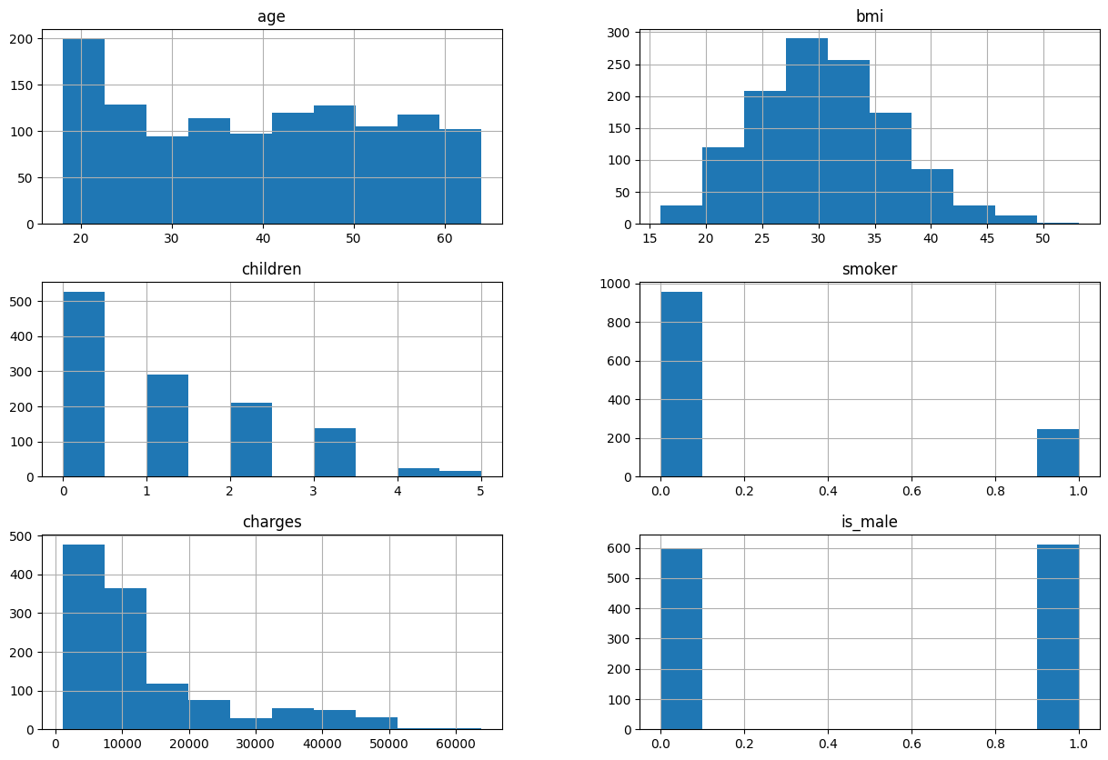
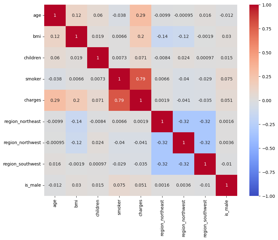
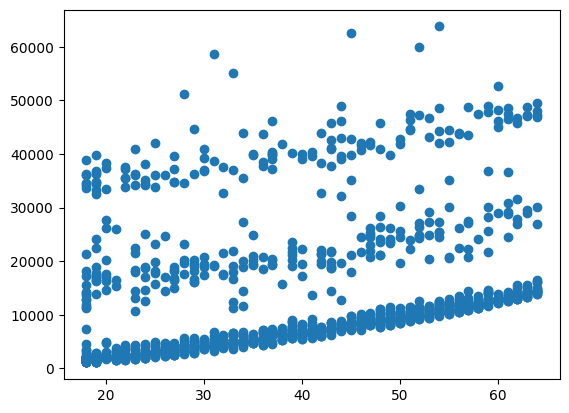
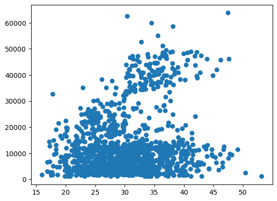
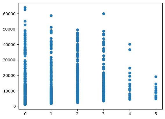
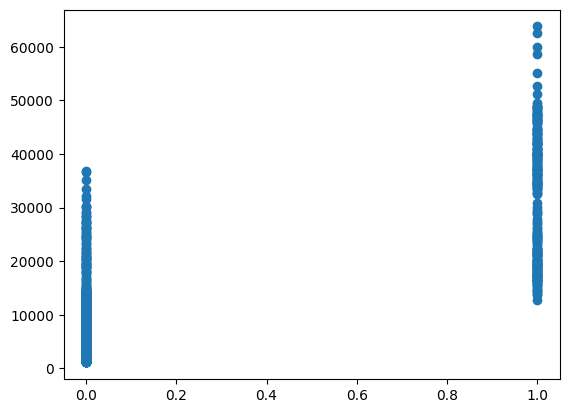
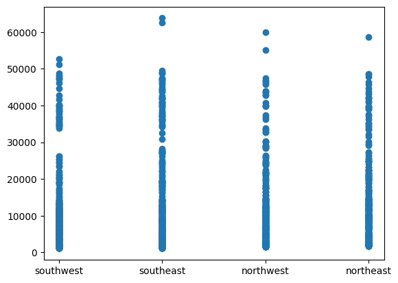
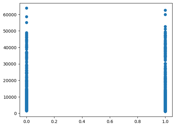
Understanding the relationships between variables is a crucial step in building predictive models. It’s important to analyze the correlations between features and the target variable (charges) to identify the most influential predictors. Visual tools such as scatter plots and heatmaps that the only strong relationship was actually found within the “Smoker” variable.
model_df.hist(figsize=(15,10))
array([[<Axes: title={'center': 'age'}>, <Axes: title={'center': 'bmi'}>],
       [<Axes: title={'center': 'children'}>,
        <Axes: title={'center': 'smoker'}>],
       [<Axes: title={'center': 'charges'}>,
        <Axes: title={'center': 'is_male'}>]], dtype=object)
plt.figure(figsize=[10,8])
sns.heatmap(model_df.corr(), annot=True, cmap="coolwarm", vmin=-1, vmax=1)
<Axes: >
plt.scatter(model_df["age"], model_df["charges"])
<matplotlib.collections.PathCollection at 0x16342d7d1d0>
plt.scatter(model_df["bmi"], model_df["charges"])
<matplotlib.collections.PathCollection at 0x1634391e990>
plt.scatter(model_df["children"], model_df["charges"])
<matplotlib.collections.PathCollection at 0x16342a4fed0>
plt.scatter(model_df["smoker"], model_df["charges"])
<matplotlib.collections.PathCollection at 0x16342a4dc10>
plt.scatter(df["region"], df["charges"])
<matplotlib.collections.PathCollection at 0x16342ada4d0>
plt.scatter(model_df["is_male"], model_df["charges"])
<matplotlib.collections.PathCollection at 0x16342ba8410>
Training the model#
To predict insurance costs, we’ll evaluate two models:
Linear Regression
A straightforward model to understand relationships in data.
Ideal for datasets with linear patterns but may struggle with complex interactions.
Random Forest Regression
A more sophisticated ensemble method that captures non-linear relationships effectively.
While powerful, it requires tuning to avoid overfitting and optimize performance.
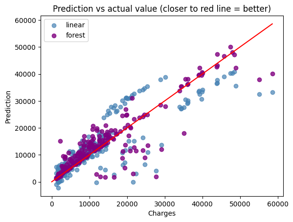
The initial results showed that Random Forest outperformed Linear Regression in terms of predictive accuracy, especially with more complex patterns.
X = model_df.drop(columns=["charges"])
y = model_df["charges"]

X_train, X_test, y_train, y_test = train_test_split(X, y, test_size=0.2, random_state=42)

model_linear = LinearRegression()
model_linear.fit(X_train, y_train)
linear_y_predict = model_linear.predict(X_test)

model_forest = RandomForestRegressor(n_jobs=1)
model_forest.fit(X_train, y_train)

forest_y_predict = model_forest.predict(X_test)

print("Initial test score")
print(f"Linear score:{model_linear.score(X_test, y_test)}")
print(f"Forest score:{model_forest.score(X_test, y_test)}")
Initial test score
Linear score:0.7049323160872817
Forest score:0.8204948228052996
cross_score_linear = cross_val_score(estimator=model_linear, X=X, y=y, scoring="r2", cv=5)
cross_score_forest = cross_val_score(estimator=model_forest, X=X, y=y, scoring="r2", cv=5)

print("Cross val score - Higher = better")
print(f"Linear score:{cross_score_linear.mean()}")
print(f"Forest score:{cross_score_forest.mean()}")
Cross val score - Higher = better
Linear score:0.7442527809757057
Forest score:0.837302077081484
r2_linear = r2_score(y_test, linear_y_predict)
r2_forest = r2_score(y_test, forest_y_predict)

print("r2 Score - Higher = better")
print(f"Linear score:{r2_linear}")
print(f"Forest score:{r2_forest}")
r2 Score - Higher = better
Linear score:0.7049323160872817
Forest score:0.8204948228052996
rmse_linear = root_mean_squared_error(y_test, linear_y_predict)
rmse_forest = root_mean_squared_error(forest_y_predict, y_test)
print("Root Mean Squared Error - Lower = better")
print(f"Linear score:{rmse_linear}")
print(f"Forest score:{rmse_forest}")
Root Mean Squared Error - Lower = better
Linear score:6319.54217986643
Forest score:4929.050667032194
mae_linear = mean_absolute_error(linear_y_predict, y_test)
mae_forest = mean_absolute_error(forest_y_predict, y_test)
print("Mean Absolute Error - Lower = better")
print(f"Linear score:{mae_linear}")
print(f"Forest score:{mae_forest}")
Mean Absolute Error - Lower = better
Linear score:4378.723562983686
Forest score:2846.14588306372
Comparing the performance#
plt.scatter(y_test, linear_y_predict, color=(70/255, 130/255, 180/255, 0.7), label="linear")
plt.scatter(y_test, forest_y_predict, color=(128/255, 0/255, 128/255, 0.8), label="forest")
plt.plot(np.linspace(0, max(y_test)), np.linspace(9, max(y_test)), color="red")
plt.xlabel("Charges")
plt.ylabel("Prediction")
plt.title("Prediction vs actual value (closer to red line = better)")
plt.legend()
<matplotlib.legend.Legend at 0x16342bf2b90>
Unveiling the feature importances#
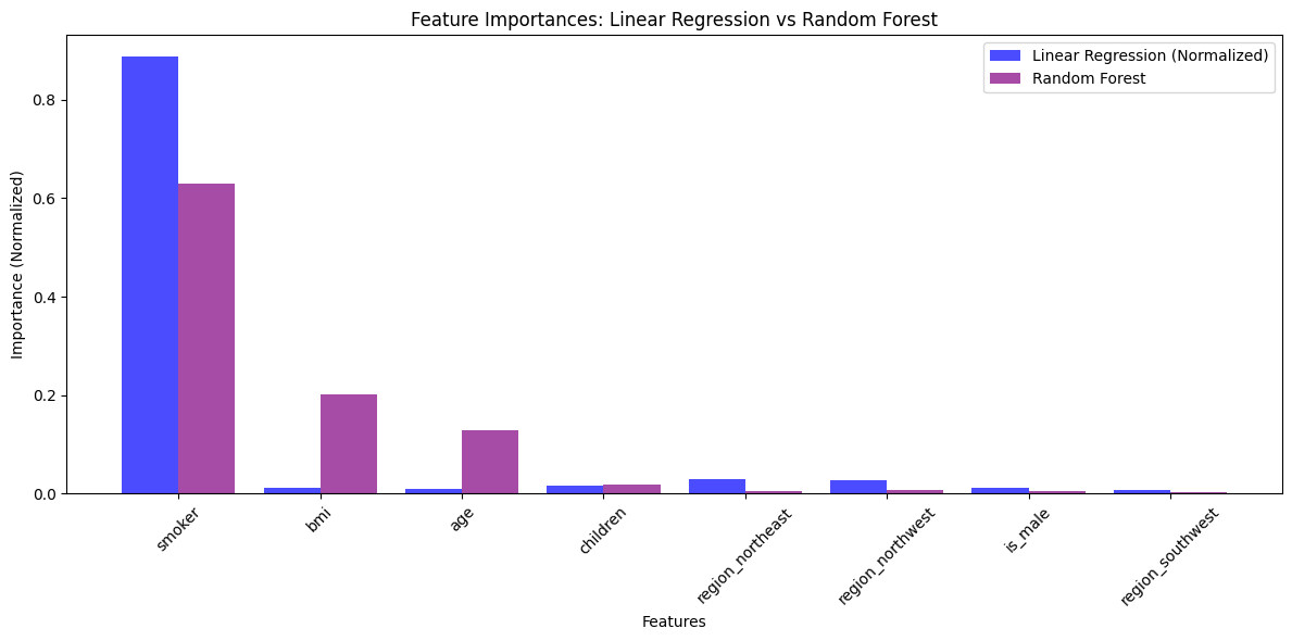
To understand which factors significantly influence insurance costs, I compared feature importances derived from the models. For this, the forest model seemed to spot weaker but relevant relationships on the variables “BMI” and “Age”.
linear_coef = model_linear.coef_
linear_importances = pd.DataFrame({
    "Feature": X_train.columns,
    "Importance": linear_coef
}).sort_values(by="Importance", key=abs, ascending=False)

# Linear refression importances
linear_total = linear_importances["Importance"].abs().sum()
linear_importance_normalized = (linear_importances["Importance"].abs() / linear_total).tolist()

linear_dict = dict(zip(linear_importances["Feature"], linear_importance_normalized))

# Random Forest Importances
forest_importances = sorted(
    zip(model_forest.feature_names_in_, model_forest.feature_importances_),
    key=lambda x: x[1],
    reverse=True
)
forest_dict = dict(forest_importances)

# Combine and sort importances
all_features = sorted(set(linear_dict.keys()).union(forest_dict.keys()))
linear_aligned = [linear_dict.get(feature, 0) for feature in all_features]
forest_aligned = [forest_dict.get(feature, 0) for feature in all_features]

combined_importance = [linear + forest for linear, forest in zip(linear_aligned, forest_aligned)]

sorted_indices = np.argsort(combined_importance)[::-1]
all_features = [all_features[i] for i in sorted_indices]
linear_aligned = [linear_aligned[i] for i in sorted_indices]
forest_aligned = [forest_aligned[i] for i in sorted_indices]

# Plot
plt.figure(figsize=(12, 6))
bar_width = 0.4
positions = np.arange(len(all_features))
plt.bar(positions - bar_width/2, linear_aligned, bar_width, label="Linear Regression (Normalized)", color="blue", alpha=0.7)
plt.bar(positions + bar_width/2, forest_aligned, bar_width, label="Random Forest", color="purple", alpha=0.7)
plt.xticks(positions, all_features, rotation=45)
plt.xlabel("Features")
plt.ylabel("Importance (Normalized)")
plt.title("Feature Importances: Linear Regression vs Random Forest")
plt.legend()

plt.tight_layout()
plt.show()
Model tuning and implementation#
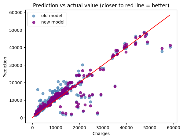
After identifying Random Forest Regression as the best-performing model, I focused on tuning its hyperparameters to maximize predictive accuracy. Key parameters like the number of trees, maximum depth, and minimum samples per leaf were adjusted using grid search and cross-validation. This process helped refine the model, reducing overfitting and improving its ability to generalize to new data.
param_grid = {
    "max_depth": [None, 2, 5, 7],
    "min_samples_split": [2, 4, 6, 8, 10],
    "min_samples_leaf": [1, 2, 4, 6, 8]
}

model = RandomForestRegressor(n_jobs=-1)

grid_search = GridSearchCV(model, param_grid=param_grid, cv=5)

grid_search.fit(X_train, y_train)
---------------------------------------------------------------------------
KeyboardInterrupt                         Traceback (most recent call last)
Cell In[27], line 11
      7 model = RandomForestRegressor(n_jobs=-1)
      9 grid_search = GridSearchCV(model, param_grid=param_grid, cv=5)
---> 11 grid_search.fit(X_train, y_train)

File ~\Documents\Projects\Analysis - Healthcare\venv\Lib\site-packages\sklearn\base.py:1473, in _fit_context.<locals>.decorator.<locals>.wrapper(estimator, *args, **kwargs)
   1466     estimator._validate_params()
   1468 with config_context(
   1469     skip_parameter_validation=(
   1470         prefer_skip_nested_validation or global_skip_validation
   1471     )
   1472 ):
-> 1473     return fit_method(estimator, *args, **kwargs)

File ~\Documents\Projects\Analysis - Healthcare\venv\Lib\site-packages\sklearn\model_selection\_search.py:1019, in BaseSearchCV.fit(self, X, y, **params)
   1013     results = self._format_results(
   1014         all_candidate_params, n_splits, all_out, all_more_results
   1015     )
   1017     return results
-> 1019 self._run_search(evaluate_candidates)
   1021 # multimetric is determined here because in the case of a callable
   1022 # self.scoring the return type is only known after calling
   1023 first_test_score = all_out[0]["test_scores"]

File ~\Documents\Projects\Analysis - Healthcare\venv\Lib\site-packages\sklearn\model_selection\_search.py:1573, in GridSearchCV._run_search(self, evaluate_candidates)
   1571 def _run_search(self, evaluate_candidates):
   1572     """Search all candidates in param_grid"""
-> 1573     evaluate_candidates(ParameterGrid(self.param_grid))

File ~\Documents\Projects\Analysis - Healthcare\venv\Lib\site-packages\sklearn\model_selection\_search.py:965, in BaseSearchCV.fit.<locals>.evaluate_candidates(candidate_params, cv, more_results)
    957 if self.verbose > 0:
    958     print(
    959         "Fitting {0} folds for each of {1} candidates,"
    960         " totalling {2} fits".format(
    961             n_splits, n_candidates, n_candidates * n_splits
    962         )
    963     )
--> 965 out = parallel(
    966     delayed(_fit_and_score)(
    967         clone(base_estimator),
    968         X,
    969         y,
    970         train=train,
    971         test=test,
    972         parameters=parameters,
    973         split_progress=(split_idx, n_splits),
    974         candidate_progress=(cand_idx, n_candidates),
    975         **fit_and_score_kwargs,
    976     )
    977     for (cand_idx, parameters), (split_idx, (train, test)) in product(
    978         enumerate(candidate_params),
    979         enumerate(cv.split(X, y, **routed_params.splitter.split)),
    980     )
    981 )
    983 if len(out) < 1:
    984     raise ValueError(
    985         "No fits were performed. "
    986         "Was the CV iterator empty? "
    987         "Were there no candidates?"
    988     )

File ~\Documents\Projects\Analysis - Healthcare\venv\Lib\site-packages\sklearn\utils\parallel.py:74, in Parallel.__call__(self, iterable)
     69 config = get_config()
     70 iterable_with_config = (
     71     (_with_config(delayed_func, config), args, kwargs)
     72     for delayed_func, args, kwargs in iterable
     73 )
---> 74 return super().__call__(iterable_with_config)

File ~\Documents\Projects\Analysis - Healthcare\venv\Lib\site-packages\joblib\parallel.py:1918, in Parallel.__call__(self, iterable)
   1916     output = self._get_sequential_output(iterable)
   1917     next(output)
-> 1918     return output if self.return_generator else list(output)
   1920 # Let's create an ID that uniquely identifies the current call. If the
   1921 # call is interrupted early and that the same instance is immediately
   1922 # re-used, this id will be used to prevent workers that were
   1923 # concurrently finalizing a task from the previous call to run the
   1924 # callback.
   1925 with self._lock:

File ~\Documents\Projects\Analysis - Healthcare\venv\Lib\site-packages\joblib\parallel.py:1847, in Parallel._get_sequential_output(self, iterable)
   1845 self.n_dispatched_batches += 1
   1846 self.n_dispatched_tasks += 1
-> 1847 res = func(*args, **kwargs)
   1848 self.n_completed_tasks += 1
   1849 self.print_progress()

File ~\Documents\Projects\Analysis - Healthcare\venv\Lib\site-packages\sklearn\utils\parallel.py:136, in _FuncWrapper.__call__(self, *args, **kwargs)
    134     config = {}
    135 with config_context(**config):
--> 136     return self.function(*args, **kwargs)

File ~\Documents\Projects\Analysis - Healthcare\venv\Lib\site-packages\sklearn\model_selection\_validation.py:888, in _fit_and_score(estimator, X, y, scorer, train, test, verbose, parameters, fit_params, score_params, return_train_score, return_parameters, return_n_test_samples, return_times, return_estimator, split_progress, candidate_progress, error_score)
    886         estimator.fit(X_train, **fit_params)
    887     else:
--> 888         estimator.fit(X_train, y_train, **fit_params)
    890 except Exception:
    891     # Note fit time as time until error
    892     fit_time = time.time() - start_time

File ~\Documents\Projects\Analysis - Healthcare\venv\Lib\site-packages\sklearn\base.py:1473, in _fit_context.<locals>.decorator.<locals>.wrapper(estimator, *args, **kwargs)
   1466     estimator._validate_params()
   1468 with config_context(
   1469     skip_parameter_validation=(
   1470         prefer_skip_nested_validation or global_skip_validation
   1471     )
   1472 ):
-> 1473     return fit_method(estimator, *args, **kwargs)

File ~\Documents\Projects\Analysis - Healthcare\venv\Lib\site-packages\sklearn\ensemble\_forest.py:489, in BaseForest.fit(self, X, y, sample_weight)
    478 trees = [
    479     self._make_estimator(append=False, random_state=random_state)
    480     for i in range(n_more_estimators)
    481 ]
    483 # Parallel loop: we prefer the threading backend as the Cython code
    484 # for fitting the trees is internally releasing the Python GIL
    485 # making threading more efficient than multiprocessing in
    486 # that case. However, for joblib 0.12+ we respect any
    487 # parallel_backend contexts set at a higher level,
    488 # since correctness does not rely on using threads.
--> 489 trees = Parallel(
    490     n_jobs=self.n_jobs,
    491     verbose=self.verbose,
    492     prefer="threads",
    493 )(
    494     delayed(_parallel_build_trees)(
    495         t,
    496         self.bootstrap,
    497         X,
    498         y,
    499         sample_weight,
    500         i,
    501         len(trees),
    502         verbose=self.verbose,
    503         class_weight=self.class_weight,
    504         n_samples_bootstrap=n_samples_bootstrap,
    505         missing_values_in_feature_mask=missing_values_in_feature_mask,
    506     )
    507     for i, t in enumerate(trees)
    508 )
    510 # Collect newly grown trees
    511 self.estimators_.extend(trees)

File ~\Documents\Projects\Analysis - Healthcare\venv\Lib\site-packages\sklearn\utils\parallel.py:74, in Parallel.__call__(self, iterable)
     69 config = get_config()
     70 iterable_with_config = (
     71     (_with_config(delayed_func, config), args, kwargs)
     72     for delayed_func, args, kwargs in iterable
     73 )
---> 74 return super().__call__(iterable_with_config)

File ~\Documents\Projects\Analysis - Healthcare\venv\Lib\site-packages\joblib\parallel.py:2007, in Parallel.__call__(self, iterable)
   2001 # The first item from the output is blank, but it makes the interpreter
   2002 # progress until it enters the Try/Except block of the generator and
   2003 # reaches the first `yield` statement. This starts the asynchronous
   2004 # dispatch of the tasks to the workers.
   2005 next(output)
-> 2007 return output if self.return_generator else list(output)

File ~\Documents\Projects\Analysis - Healthcare\venv\Lib\site-packages\joblib\parallel.py:1650, in Parallel._get_outputs(self, iterator, pre_dispatch)
   1647     yield
   1649     with self._backend.retrieval_context():
-> 1650         yield from self._retrieve()
   1652 except GeneratorExit:
   1653     # The generator has been garbage collected before being fully
   1654     # consumed. This aborts the remaining tasks if possible and warn
   1655     # the user if necessary.
   1656     self._exception = True

File ~\Documents\Projects\Analysis - Healthcare\venv\Lib\site-packages\joblib\parallel.py:1762, in Parallel._retrieve(self)
   1757 # If the next job is not ready for retrieval yet, we just wait for
   1758 # async callbacks to progress.
   1759 if ((len(self._jobs) == 0) or
   1760     (self._jobs[0].get_status(
   1761         timeout=self.timeout) == TASK_PENDING)):
-> 1762     time.sleep(0.01)
   1763     continue
   1765 # We need to be careful: the job list can be filling up as
   1766 # we empty it and Python list are not thread-safe by
   1767 # default hence the use of the lock

KeyboardInterrupt:
grid_search.best_params_
{'max_depth': 5, 'min_samples_leaf': 8, 'min_samples_split': 10}
Comparing the trained and untrained model#
model = grid_search.best_estimator_
model_y_predict = model.predict(X_test)

print("Initial test score")
print(f"Old model score:{model_forest.score(X_test, y_test)}")
print(f"New model score:{model.score(X_test, y_test)}")
Initial test score
Old model score:0.8206838233843838
New model score:0.8492189951744393
rmse_model = root_mean_squared_error(model_y_predict, y_test)
print("Cross val score - Higher = better")
print(f"Old model score:{rmse_forest}")
print(f"New model score:{rmse_model}")
Cross val score - Higher = better
Old model score:4926.455090703199
New model score:4517.49946296272
mae_model = mean_absolute_error(forest_y_predict, y_test)
print("Mean Absolute Error - Lower = better")
print(f"Old model score:{mae_forest}")
print(f"New model score:{mae_model}")
Mean Absolute Error - Lower = better
Old model score:2890.690395782397
New model score:2890.690395782397
plt.scatter(y_test, forest_y_predict, color=(70/255, 130/255, 180/255, 0.7), label="old model")
plt.scatter(y_test, model_y_predict, color=(128/255, 0/255, 128/255, 0.8), label="new model")
plt.plot(np.linspace(0, max(y_test)), np.linspace(9, max(y_test)), color="red")
plt.xlabel("Charges")
plt.ylabel("Prediction")
plt.title("Prediction vs actual value (closer to red line = better)")
plt.legend()
<matplotlib.legend.Legend at 0x261d64fbed0>
Model implementation#
Lastly, here’s an implementation of the model in another dataset.
validation_df = pd.read_csv("validation_dataset.csv")
validation_df = pd.get_dummies(df, prefix=["region"], columns=["region"])
validation_df = validation_df.drop(columns=["region_southeast"])

validation_df["smoker"] = (validation_df["smoker"] == "yes")
validation_df["smoker"] = validation_df["smoker"].astype("int64")

validation_df["is_male"] = (validation_df["sex"] == "male").astype("int64")

validation_df = validation_df.drop(columns=["sex", "charges"])

validation_df = validation_df.dropna()

validation_df.head()
| age | bmi | children | smoker | region_northeast | region_northwest | region_southwest | is_male | |
|---|---|---|---|---|---|---|---|---|
| 0 | 19.0 | 27.900 | 0.0 | 0 | False | False | True | 0 |
| 1 | 18.0 | 33.770 | 1.0 | 0 | False | False | False | 1 |
| 2 | 28.0 | 33.000 | 3.0 | 0 | False | False | False | 1 |
| 3 | 33.0 | 22.705 | 0.0 | 0 | False | True | False | 1 |
| 4 | 32.0 | 28.880 | 0.0 | 0 | False | True | False | 1 |
predictions = model.predict(validation_df)

validation_df["predicted_charges"] = predictions

validation_df.loc[validation_df["predicted_charges"] < 1000, "predicted_charges"] = 1000

validation_df
| age | bmi | children | smoker | region_northeast | region_northwest | region_southwest | is_male | predicted_charges | |
|---|---|---|---|---|---|---|---|---|---|
| 0 | 19.0 | 27.900 | 0.0 | 0 | False | False | True | 0 | 2480.767194 |
| 1 | 18.0 | 33.770 | 1.0 | 0 | False | False | False | 1 | 2949.559493 |
| 2 | 28.0 | 33.000 | 3.0 | 0 | False | False | False | 1 | 6088.056232 |
| 3 | 33.0 | 22.705 | 0.0 | 0 | False | True | False | 1 | 7212.123538 |
| 4 | 32.0 | 28.880 | 0.0 | 0 | False | True | False | 1 | 5087.370942 |
| ... | ... | ... | ... | ... | ... | ... | ... | ... | ... |
| 1203 | 50.0 | 30.970 | 3.0 | 0 | False | True | False | 1 | 10909.637490 |
| 1204 | 18.0 | 31.920 | 0.0 | 0 | True | False | False | 0 | 3304.237192 |
| 1205 | 18.0 | 36.850 | 0.0 | 0 | False | False | False | 0 | 2452.888815 |
| 1206 | 21.0 | 25.800 | 0.0 | 0 | False | False | True | 0 | 2516.053311 |
| 1207 | 61.0 | 29.070 | 0.0 | 0 | False | True | False | 0 | 13942.487977 |
1208 rows × 9 columns
Conclusion and Closing#
Thank you for taking the time to explore this project with me. From data preparation to model validation, We’ve walked through the process of building a predictive model for insurance costs, highlighting key steps like cleaning data, comparing models, and fine-tuning performance.
If you have any questions or would like to dive deeper into specific aspects of the project, I’d be happy to assist!
You can contact me at [business@falcontreras.com] or alternatively there’s a contact form within falcontreras.com
Thank you! 👋
